Some Numerical Results for Zero Boundary Conditions Along the y-Axis
By Linda Stals
A study of the nonlinear behaviour of the Hasegawa-Wakatani equations has been carried out and documented in arXiv:1107.0112. Here we include some additional simulations highlighting the results for periodic boundary conditions along the x-axis and zero boundary conditions along the y-axis.
We found that if both axis have periodic boundary conditions, the (0, ± 1) modes are unstable. If zero boundary conditions are applied to the y-axis, these unstable modes are removed from the system. Eigenvalue analysis of the linear system of equations suggests that the modes along the x-axis will always be stable.
A low mode analysis carried out with aid of the centre manifold showed that for certain choice of parameters, the (±1, ± 1) modes are unstable. However, as additional modes are included in the simulations evidence of bifurcation behaviour becomes apparent. Additional simulations were carried out for βr = β&phi = 0.001, 0.00001 and 0.0000001.
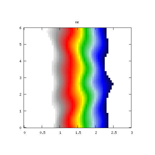
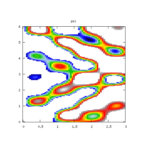
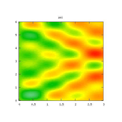
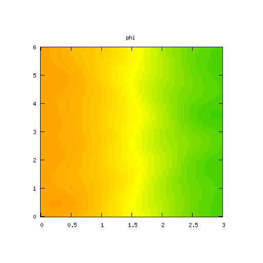
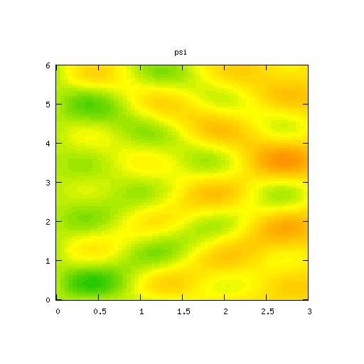
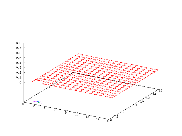
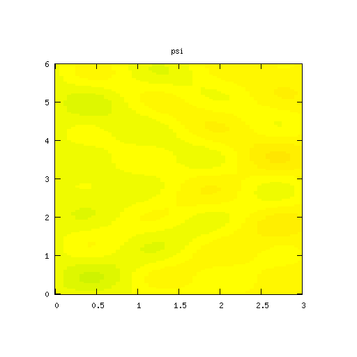
The three movies below show how the potential φ, density r and vorticity ∇2 φ change with time. The grid size is [0,2π/k]×[0, 2π/k] where k = 1. Click on the image to enlarge. For the Fourier mode simulations, we have only shown a 16×16 section of grid, the actual computational domain may be higher.
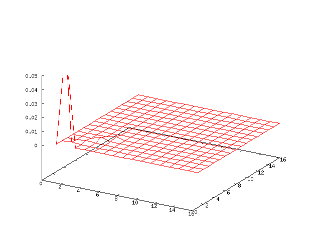
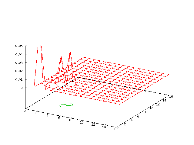
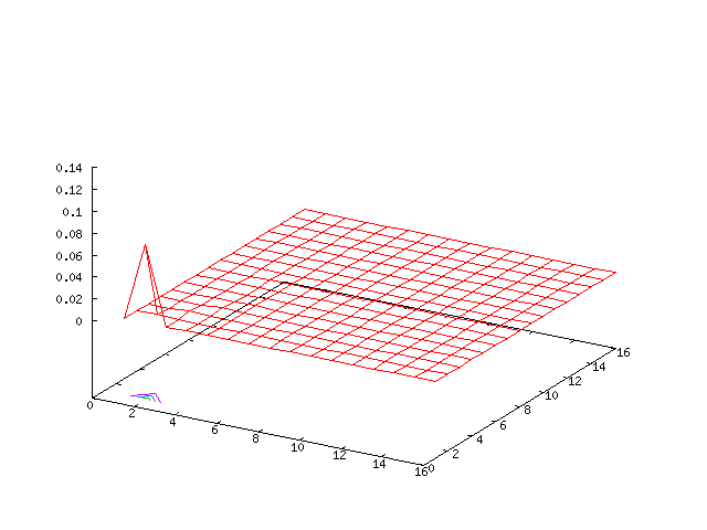
Low Mode Example
Results for
According to the low mode analysis, the modes along the x-axis should be damped out, but the (±1, ± 1) modes will, eventually, grow exponentially.
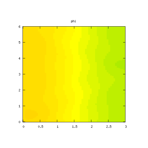
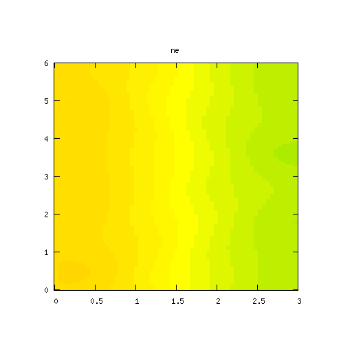
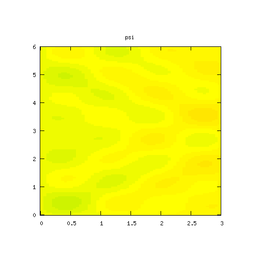
| Potential | Density | Vorticity |

|
|
|
| Potential | Density | Vorticity |

|
|
|
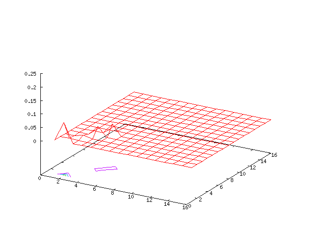
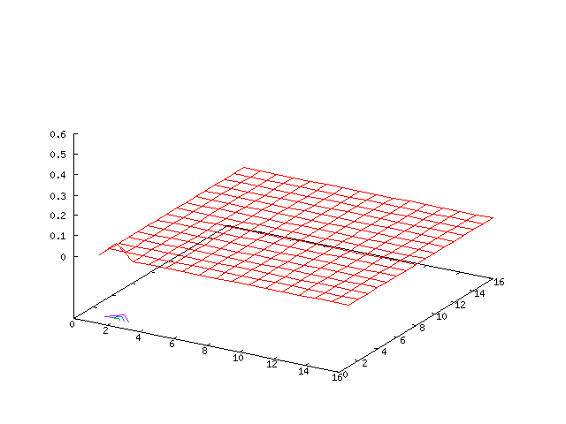
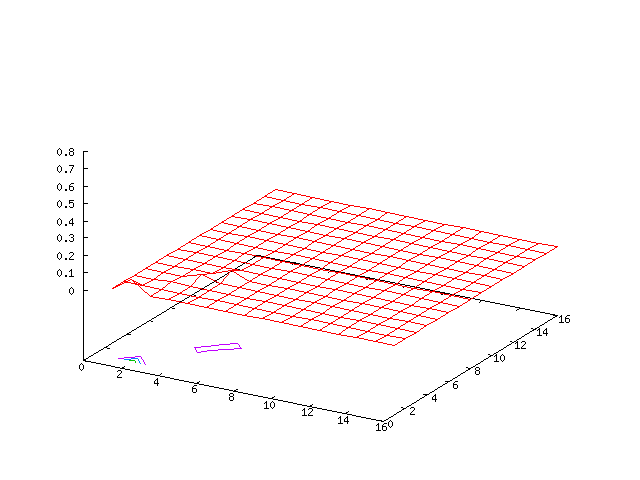
High Mode Example
Results for p = 2, βr = β&phi = 0.01, κ = 1.0, α = 1, 0 ≤ t ≤ 5000 and computational grid size = 128 × 128
We expect to see a growth in the (± 1, ± 1) modes, but the modes along the x-axis are damped out. With the right choice of parameters, the interactions between these modes balance one another out to give stable bifurcation behaviour.
| Potential | Density | Vorticity |

|
|
|
| Potential | Density | Vorticity |

|

|
|
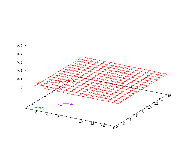
High Mode Example, βr = β&phi = 0.001
Results for p = 2, βr = β&phi = 0.001, κ = 1.0, α = 1, 0 ≤ t ≤ 5000 and computational grid size = 128 × 128
The interaction between the growth in the (± 1, ± 1) modes and the dampening of the modes along the x-axis is particularly evident in this example.
| Potential | Density | Vorticity |

|

|
|
| Potential | Density | Vorticity |
|

|
|
High Mode Example, βr = β&phi = 0.00001
Results for p = 2, βr = β&phi = 0.00001, κ = 1.0, α = 1, 0 ≤ t ≤ 5000 and computational grid size = 128 × 128
By reducing the value of βr and β&phi additional modes influence the long-term behaviour of the system, but the lower order modes still dominate.
| Potential | Density | Vorticity |
|

|
|
| Potential | Density | Vorticity |
|
|
|
High Mode Example, βr = β&phi = 0.0000001
Results for p = 2, βr = β&phi = 0.0000001, κ = 1.0, α = 1, 0 ≤ t ≤ 5000 and computational grid size = 128 × 128
The final example looks at the simulation results for small values of βr and β&phi.
| Potential | Density | Vorticity |
|

|

|
| Potential | Density | Vorticity |

|

|
|