The thin-plate spline for a general domain Ω, as formulated by Wahba [2] and Duchon [1], is the function, f, that minimises the functional

Jα(f) = 1 n n ∑ i=1  (f(x(i))−y(i))2 + α ⌠ ⌡ Ω  ∑ |ν|=2      2 ν     ( Dν f(x) )2 dx,

(1)

where ν = (ν₁,...,ν_d) is a d dimensional multi-index, |ν| = ∑_s=1^d ν_s, x is a predictor variable in R^d, and x⁽ⁱ⁾ and y⁽ⁱ⁾ are the corresponding i-th predictor and response data value (1 ≤ i ≤ n). The smoothing parameter α controls the trade-off between smoothness and fit. In the limit α→ 0 the function f becomes an interpolant. If α is large, f becomes very smooth but may not reflect the data very well. The value of α may be automatically calculated using generalised cross validation [2]. Radial basis functions are often used to represent f as they give an analytical solution to the minimiser of the functional in Equation (1). The system of equations resulting from the radial basis functions is dense and its size is directly proportional to the number of data points. In applications with a large number of data points the system is very expensive to compute. We propose a discrete thin-plate spline method that uses polynomial basis function with local support defined on a finite element mesh. The resulting system of equations is sparse and its size depends only on the number of grid points in the finite element mesh. A preconditioned conjugate gradient (CG) method is used to solve the system of equations. The smoothing problem from Equation (1) can be approximated with finite elements so that the discrete smoother f is a piecewise multi-linear function. In vector notation f will be of the form

f(x)=b(x)Tc.

The idea is to minimise J_α over all f of this form. The smoothing term is not defined for piecewise multi-linear functions, but the non-conforming finite element principle can be used to introduce piecewise multi-linear functions u = (b^Tg₁,...,b^Tg_d) to represent the gradient of f. The functions f and u satisfy the relationship

⌠ ⌡ Ω  ∇f(x) ·∇v(x) dx = ⌠ ⌡ Ω  u(x) ·∇v(x) dx,

(2)

for all piecewise multi-linear function v. This is equivalent to the relationship

L c = d ∑ s=1  Gs gs,

(3)

where L is a discrete approximation to the negative Laplace operator and (G₁ ,..., G_d) is a discrete approximation to the transpose of the gradient operator. We now consider the minimiser of the functional

Jα(c,g1,...,gd) = 1 n n ∑ i=1  (b(x(i))Tc−y(i))2 + α ⌠ ⌡ Ω  d ∑ s=1  ∇(bT gs)·∇(bT gs) dx = 1 n n ∑ i=1  (b(x(i))Tc−y(i))2 + α d ∑ s=1  gsT L gs . (4)

Our smoothing problem consists of minimising this functional over all vectors c, g₁,...,g_d, defined on the domain Ω_h, subject to the Constraint (3). In the 3D case the discrete minimisation problem (4) is equivalent to finding the minimum of

Jα(c,g1, g2, g3) = cT A c − 2dTc + yTy/n + α(g1T L g1 + g2T L g2 + g3T L g3),

(5)

subject to

L c − G1 g1 − G2 g2 − G3 g3 = 0.

(6)

The matrices L, G₁, G₂ and G₃ are independent of the data points but the matrix

A = 1 n n ∑ i=1  b(x(i))b(x(i))T,

and vector

d = 1 n n ∑ i=1  b(x(i))y(i),

must be assembled by sweeping through the data points. The matrix A is symmetric indefinite and sparse. By using Lagrange multipliers Minimisation Problem (5) may be rewritten as the solution of the linear system:

        A 0 0 0 L 0 αL 0 0 −G1T 0 0 αL 0 −G2T 0 0 0 αL −G3T L −G1 −G2 −G3 0                 c g1 g2 g3 w         =         d 0 0 0 0         ,

(7)

where w is a Lagrange multiplier associated with Constraint (6). We have assumed zero Dirichlet boundary conditions. One way to solve Equation (7) is to eliminate all of the variables except g₁, g₂ and g₃, which gives

     αL + G1T Z G1 G1T Z G2 G1T Z G3 G2T Z G1 αL + G2T Z G2 G2T Z G3 G3T Z G1 G3T Z G2 αL + G3T Z G3           g1 g2 g3      =      G1T L−1d G2T L−1d G3T L−1d      ,

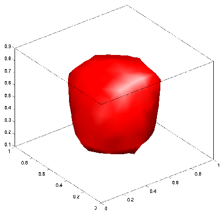
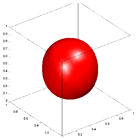
where Z = L⁻¹A L⁻¹ and c = L⁻¹(G₁ g₁ + G₂ g₂ + G₃ g₃ −h₅ ). We now briefly present some examples of data fitting in 3D. Iso-surface plot of the sphere on a grid with 189 and 68705 nodes. The first data set contained 10⁶ points generated randomly on a sphere with centre (0.5, 0.5, 0.5) and radius 1/3. The data points were assigned a value of 1. The smoothing parameter α was set to 10⁻³. Figure 1 shows an Iso-surface plot of the discrete thin plate spline with 189 nodes and 68705 nodes respectively. 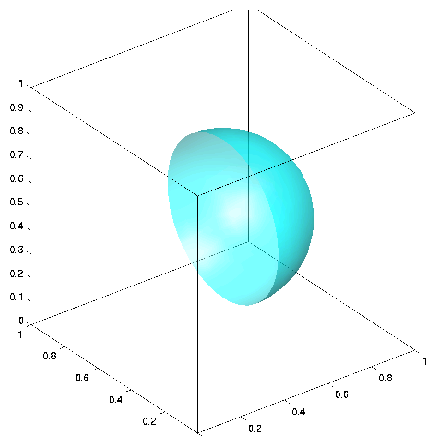Iso-surface representation of the original data set for the semi-sphere example and approximation on a grid with 68705 nodes. The next data set is designed to represent the case where there is missing data. Specifically, we took the data from the example described above and removed all of those points with x-coordinate less than 0.5. See Figure 2. The data set contained approximately 1/2 ×10⁶ points. Note that the spline attempted to fill in the missing data. The value for α was set to 10⁻³. 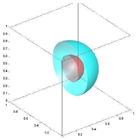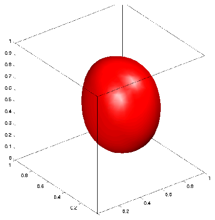Iso-surface representation of the original data set for the semi-sphere example with an additional layer of data points placed in the interior and the approximation on a grid with 68705 nodes. In the final example an inner layer of data points were added to force the discrete thin plate spline approximation to more closely follow the shape of the semi-sphere. Along with the data points from the previous example, additional data points sitting on the semi-sphere with centre (0.5, 0.5, 0.5) and radius = 1/6 were added and given a value of 0. See Figure 3. There are approximately 2×(1/2 ×10⁶) data points. The smoothing parameter, α, was reduced to 10⁻⁷.

References

[1]

J. Duchon, Splines minimizing rotation-invariant., in Lecture Notes in Math, vol. 571, Springer-Verlag, 1977, pp. 85-100.

[2]

G. Wahba, Spline models for observational data, vol. 59 of CBMS-NSF Regional Conference Series in Applied Mathematics, Society for Industrial and Applied Mathematics (SIAM), Philadelphia, PA, 1990.

---

File translated from T_EX by T_TH, version 3.67.
On 12 Oct 2005, 23:18.